🚀 The Catalyst Optimizer

In our last post, we learned about Lazy Evaluation: Spark waits until the last moment to execute so it can build a "plan."

But how is that plan built? And how does Spark know that "filtering before joining" is faster than "joining before filtering"?

Meet the Catalyst Optimizer.

If RDDs are the muscle and DataFrames are the API, Catalyst is the brain. It is the engine that takes your messy, unoptimized code and rewrites it into an efficient execution plan.

The Workflow: From Query to RDDs

The diagram below shows the journey of your code. Every time you run a DataFrame transformation, Catalyst guides it through these four phases before a single task is launched on the cluster .

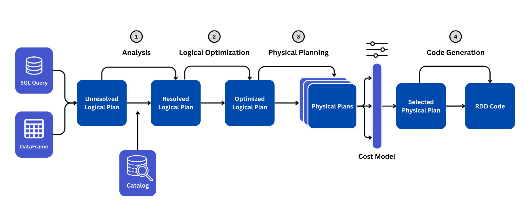
Phase 1: Analysis (Unresolved → Logical Plan)

When you type df.select("name"), Spark doesn't know if "name" exists or if it's a typo.

• The Unresolved Logical Plan: Spark reads your code but hasn't checked validity yet.
• The Catalog: Catalyst looks up the Table/DataFrame metadata.
• Resolution: It confirms: "Does column 'name' exist? Is it a string or int?" If correct, it creates the Logical Plan.

Phase 2: Logical Optimization (The "Rule" Book)

This is where the magic happens. Catalyst applies a set of standard rules to optimize your logic without caring about physical servers or data size yet.

• Predicate Pushdown: Moves filter() commands as close to the data source as possible.
• Projection Pruning: Removes columns you didn't select early in the chain.
• Constant Folding: Converts col("salary") * (100 + 10) → col("salary") * 110.
• Boolean Simplification: Simplifies filter(TRUE and condition) to filter(condition).

Result: An Optimized Logical Plan.

Phase 3: Physical Planning (The Strategy)

Now Spark knows what to do, but not how to do it. The Physical Planner generates multiple strategies to execute the logic.

• "Should I join these tables using a Sort Merge Join or a Broadcast Hash Join?"
• "Should I scan the whole file or use an index?"

The Cost Model: Spark estimates the "cost" (CPU, IO) of each strategy and picks the cheapest one. This is the Selected Physical Plan.

Phase 4: Code Generation (Tungsten)

Once the plan is finalized, you might think Spark runs it interpretively (like standard Python). It does not. Spark uses a feature called Whole-Stage Code Generation (powered by Project Tungsten). It collapses the entire query plan into a single, highly optimized Java function (Bytecode) that runs directly on the CPU, removing the overhead of function calls.

This is why PySpark is almost as fast as Scala - the Python code is just a wrapper to generate this final Java bytecode!

Example: Catalyst in Action

Let’s trace a simple query through the phases.

Your Code:

df1 = spark.read.csv("users.csv")
df2 = spark.read.csv("orders.csv")
joined = df1.join(df2, "user_id").filter(df2["amount"] > 100)

1. Analysis: Checks if users.csv and orders.csv exist and have user_id/amount.
2. Logical Optimization:
   • Bad Plan: Join all users and orders (Shuffle huge data), THEN filter for amount > 100.
   • Optimized Plan (Predicate Pushdown): Filter orders for amount > 100 FIRST, then Join. (Drastically reduces data size).
3. Physical Planning:
   • Strategy A: Shuffle both large tables (SortMergeJoin).
   • Strategy B: If users is tiny, send it to every node (BroadcastJoin).
   • Selection: Spark checks the file size. If users < 10MB, it picks Strategy B (Broadcast).
4. Code Gen: Creates a single Java function to read, filter, hash, and join in one pass.

How to See the DAG Plans in PySpark

Spark provides two primary ways to inspect the Catalyst Optimizer's work: the programmatic explain() method and the visual Spark UI.

1. The explain() Method

The quickest way to see the plan is by calling the .explain() method on any DataFrame. By default, this prints only the Physical Plan, which is the final strategy Spark has selected for execution.

To see the full journey—from the unresolved code to the optimized strategy—you should use the mode="extended" parameter.

# Standard Physical Plan (Default)
df.explain()

# The Full Journey (Parsed, Analyzed, Optimized, Physical)
df.explain(mode="extended")

# A Cleaner, Formatted View of the Physical Plan
df.explain(mode="formatted")

When you run mode="extended", the output mirrors the four phases we discussed:

• Parsed Logical Plan: Your code as written (Unresolved).
• Analyzed Logical Plan: Metadata resolved against the Catalog.
• Optimized Logical Plan: After rules like Predicate Pushdown are applied.
• Physical Plan: The specific strategy (e.g., BroadcastHashJoin) chosen by the Cost Model.

2. The Spark UI (SQL Tab)

For complex queries, text output can be hard to read. The Spark UI provides a visual Directed Acyclic Graph (DAG) of the plan.

1. Open the Spark UI (usually on port 4040 locally or the "Compute" tab in Databricks).
2. Navigate to the SQL / DataFrame tab.
3. Click on the description of your latest query (e.g., "collect at ").

This view visualizes the Physical Plan as a flowchart. You will see boxes representing operations like Scan csv, Filter, and Exchange (Shuffle). If you see a box labeled WholeStageCodegen, that indicates Tungsten has successfully collapsed multiple operations into a single optimized function.

---

Decoding the Plan Output

Let's look at the plan for a simple aggregation. In this example, we load customer data, group by city, and count the users. You can also try to run this code and test it in our PySpark Online Compiler.

The Code:

df = spark.read.format('csv').option('header', 'true').load('/samples/customers.csv')
df = df.groupBy('city').count()
df.explain(mode='extended')

The Output:

== Parsed Logical Plan ==
'Aggregate ['city], ['city, count(1) AS count#2565L]
+- Relation [customer_id#2537,first_name#2538,last_name#2539,email#2540,phone_number#2541,address#2542,city#2543,state#2544,zip_code#2545] csv

== Analyzed Logical Plan ==
city: string, count: bigint
Aggregate [city#2543], [city#2543, count(1) AS count#2565L]
+- Relation [customer_id#2537,first_name#2538,last_name#2539,email#2540,phone_number#2541,address#2542,city#2543,state#2544,zip_code#2545] csv

== Optimized Logical Plan ==
Aggregate [city#2543], [city#2543, count(1) AS count#2565L]
+- Project [city#2543]
   +- Relation [customer_id#2537,first_name#2538,last_name#2539,email#2540,phone_number#2541,address#2542,city#2543,state#2544,zip_code#2545] csv

== Physical Plan ==
AdaptiveSparkPlan isFinalPlan=false
+- HashAggregate(keys=[city#2543], functions=[count(1)], output=[city#2543, count#2565L])
   +- Exchange hashpartitioning(city#2543, 200), ENSURE_REQUIREMENTS, [plan_id=1823]
      +- HashAggregate(keys=[city#2543], functions=[partial_count(1)], output=[city#2543, count#2570L])
         +- FileScan csv [city#2543] Batched: false, DataFilters: [], Format: CSV, Location: InMemoryFileIndex(1 paths)[file:/samples/customers.csv], PartitionFilters: [], PushedFilters: [], ReadSchema: struct<city:string>

Here is what that scary wall of text actually means, broken down by phase.

1. Parsed & Analyzed: "The Understanding"

== Parsed Logical Plan ==
'Aggregate ['city], ['city, count(1) AS count#2565L]
+- Relation [customer_id#2537,first_name#2538,last_name#2539,email#2540,phone_number#2541,address#2542,city#2543,state#2544,zip_code#2545] csv

== Analyzed Logical Plan ==
city: string, count: bigint
Aggregate [city#2543], [city#2543, count(1) AS count#2565L]
+- Relation [customer_id#2537,first_name#2538,last_name#2539,email#2540,phone_number#2541,address#2542,city#2543,state#2544,zip_code#2545] csv

• What happened: Spark successfully looked up the schema.
• The clues: Notice city: string, count: bigint. In the "Parsed" step, it didn't know these types yet. Now, it has confirmed that city exists in the CSV and is a string.
• Note on IDs: See those numbers like #2543? Those are internal unique IDs Spark assigns to every column to track them, even if you rename them later.

2. Optimized: "The Pruning"

== Optimized Logical Plan ==
Aggregate [city#2543], [city#2543, count(1) AS count#2565L]
+- Project [city#2543]
   +- Relation [customer_id#2537,first_name#2538,last_name#2539,email#2540,phone_number#2541,address#2542,city#2543,state#2544,zip_code#2545] csv

• The Magic: We never told Spark to select only the city column. We just ran a groupBy.
• The Optimization: Catalyst realized that to count users by city, it does not need email, phone_number, or address.
• Project [city]: It inserted a Project (Select) operation to effectively drop all other columns immediately. This is Column Pruning in action, saving massive amounts of memory.

3. Physical: "The Execution Strategy"

The Physical Plan is read from the bottom up.

== Physical Plan ==
AdaptiveSparkPlan isFinalPlan=false
+- HashAggregate(keys=[city#2543], functions=[count(1)], output=[city#2543, count#2565L])
   +- Exchange hashpartitioning(city#2543, 200), ENSURE_REQUIREMENTS, [plan_id=1823]
      +- HashAggregate(keys=[city#2543], functions=[partial_count(1)], output=[city#2543, count#2570L])
         +- FileScan csv [city#2543] Batched: false, DataFilters: [], Format: CSV, Location: InMemoryFileIndex(1 paths)[file:/samples/customers.csv], PartitionFilters: [], PushedFilters: [], ReadSchema: struct<city:string>

1. FileScan csv: Spark reads the file. Notice ReadSchema: struct<city:string>. Because of the optimization step above, it physically only pulls the city column from the disk.
2. HashAggregate (partial_count): This is a huge performance booster. Spark counts the cities on the local partition first (e.g., "I found 5 users in Chicago on this node").
3. Exchange (Shuffle): Now, it must move data so that all "Chicago" records end up on the same node. This is the heavy lifting.
4. HashAggregate (count): Finally, it sums up the partial counts from all nodes to get the total.

A Note on AdaptiveSparkPlan

You can see on the very first line of the Physical Plan:

== Physical Plan ==
AdaptiveSparkPlan isFinalPlan=false

This indicates that Adaptive Query Execution (AQE) is active.

• isFinalPlan=false: This means the plan you see is just the initial strategy. As the job runs, Spark will monitor the actual data size. If the data turns out to be different than estimated (e.g., much smaller after filtering), AQE can pause execution and re-optimize the plan on the fly to be more efficient.

It is a powerful feature that deserves its own spotlight. We will be diving deep into AQE and how it dynamically fixes query performance in the upcoming posts!

Summary

Phase	Input	What Happens?
Analysis	Code / SQL	Checks column names, types, and table existence.
Logical Opt	Resolved Plan	Reorders operations (Pushdown, Pruning) for efficiency.
Physical Plan	Optimized Plan	Selects algorithms (Hash Join vs Sort Merge, Broadcast).
Code Gen	Physical Plan	Compiles logic into raw Java Bytecode (Tungsten) for speed.

Note - we have also introduced some terms here like Hash, Sort Merge, and Broadcast Joins. We'll be diving into these in the later posts.

---